

MATCH is the quiet workhorse behind many smart spreadsheets. Instead of returning a value, it tells you *where* that value lives in a list or table. That position becomes the key that other formulas use: INDEX to pull prices, regions, owners; SUM or OFFSET to aggregate the right slice of data; or validation checks to flag mismatches. In both Excel and Google Sheets, MATCH supports exact, approximate, and wildcard searches, making it ideal for messy real-world lists of products, contacts, or transactions. When your business logic depends on “find the right row, then do X,” MATCH is usually step one.Now imagine never touching those formulas again. An AI computer agent watches your Google Sheets and Excel workbooks, learns your matching patterns, and then takes over: building INDEX+MATCH formulas, testing 0 vs 1 match_type, handling #N/A errors, and updating ranges as your lists grow. Instead of hunting through columns yourself, you just describe the outcome—“match these new orders to our master SKU list”—and the agent drives the spreadsheet for you.
If you run a sales team, agency, or operations-heavy business, you already live inside spreadsheets. MATCH is one of those functions that quietly runs half your reports. But most teams either underuse it or bury it in fragile formulas that break whenever someone inserts a new column.In this guide, we’ll walk through three layers of mastery:1) Manual MATCH techniques you should know cold.2) No‑code automation to reduce copy‑paste drudgery.3) How to let an AI agent operate MATCH at scale across Google Sheets and Excel.### 1. Manual ways to use MATCH (the foundations)These are the building blocks your team should understand before you automate anything.**1. Basic exact MATCH for IDs (Excel and Sheets)**
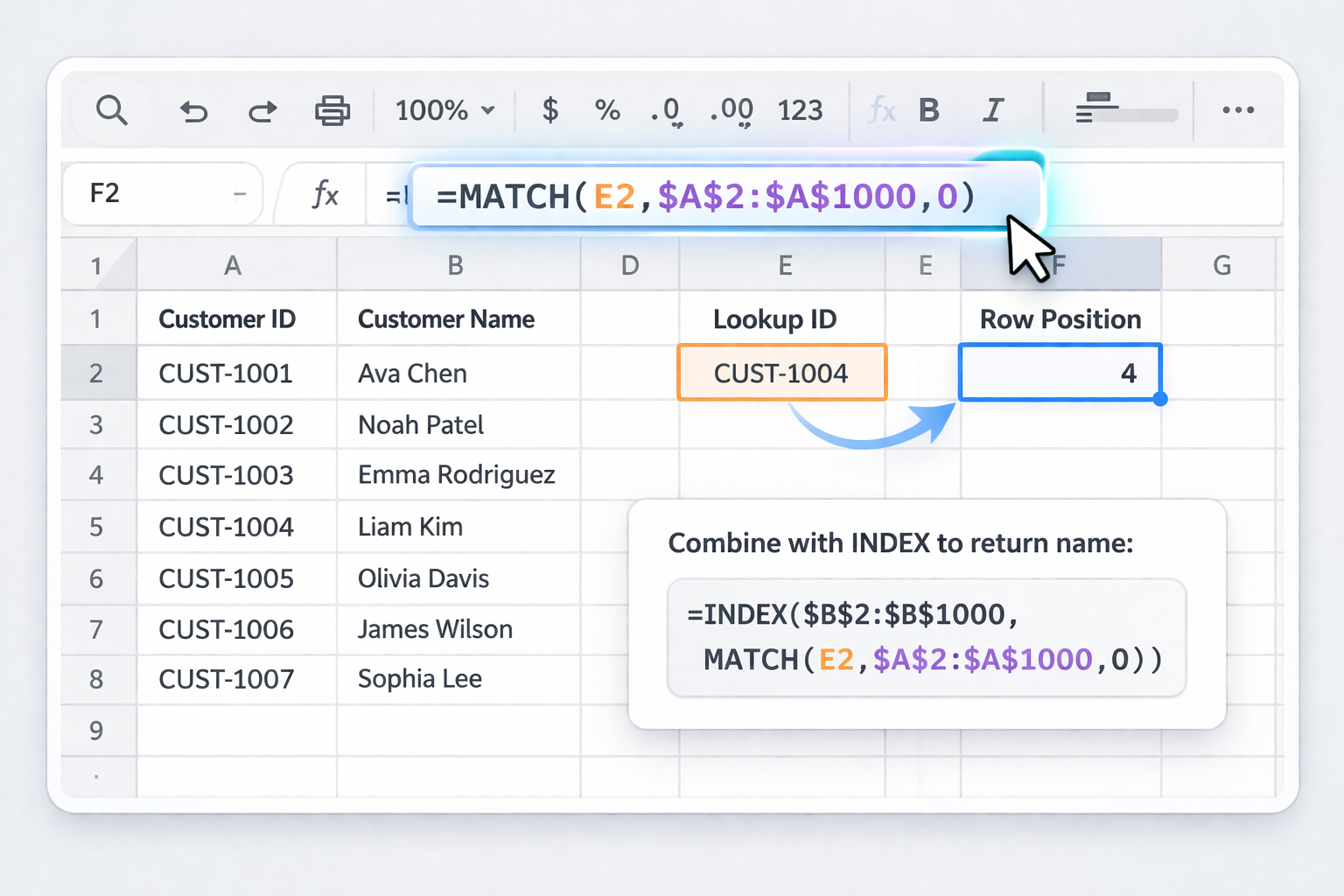
Goal: Find the row position of a customer ID in a master list.1. Put your lookup value in a cell, e.g. `E2`.2. In Excel, use: `=MATCH(E2,$A$2:$A$1000,0)`3. In Google Sheets, use the same: `=MATCH(E2,$A$2:$A$1000,0)`4. The result is the row *position* within the range, not the row number on the sheet.5. Combine with INDEX to pull a value: `=INDEX($B$2:$B$1000, MATCH(E2,$A$2:$A$1000,0))` to get, say, the customer name.Official docs:- Excel MATCH: https://support.microsoft.com/en-us/office/match-function-e8dffd45-c762-47d6-bf89-533f4a37673a- Sheets INDEX+MATCH guide: https://support.google.com/docs/answer/3093378**2. Approximate MATCH for pricing tiers or bands**Great for volume-based discounts or commission tiers.1. Create a table of thresholds in ascending order, e.g. quantities in `A2:A10`, discount % in `B2:B10`.2. In your invoice row, with quantity in `E2`, use: `=MATCH(E2,$A$2:$A$10,1)`3. This returns the position of the largest value less than or equal to `E2`.4. Wrap with INDEX to get the correct discount: `=INDEX($B$2:$B$10, MATCH(E2,$A$2:$A$10,1))`5. Remind your team: data MUST be sorted ascending for match_type 1.**3. Wildcard MATCH for messy text lists**For lead lists where company names are inconsistent.1. Suppose you have company names in `A2:A500`.2. In a helper cell, type a flexible search pattern like `"*Acme*"`.3. Use: `=MATCH("*Acme*",$A$2:$A$500,0)`4. MATCH returns the position of the first name containing “Acme”.5. Use INDEX to pull related columns (owner, stage, MRR) from the same row.**4. Two‑way lookup with INDEX+MATCH (rows and columns)**Useful for revenue by region and month.1. Regions in `A2:A10`, months across `B1:M1`, data in `B2:M10`.2. Region in `P1`, month in `P2`.3. Row position: `=MATCH(P1,$A$2:$A$10,0)`4. Column position: `=MATCH(P2,$B$1:$M$1,0)`5. Final lookup: `=INDEX($B$2:$M$10, MATCH(P1,$A$2:$A$10,0), MATCH(P2,$B$1:$M$1,0))`Train your team to always specify match_type (0, 1 or -1) explicitly to avoid silent errors.### 2. No‑code automation methodsOnce the basics are in place, you can reduce manual formula work using built-in automation.**A. Use named ranges and templates**Instead of hard‑coding ranges, define named ranges like `Leads_IDs` or `SKU_List`. In Excel (Formulas > Name Manager) and in Sheets (Data > Named ranges), configure names that auto-expand as you add rows.Then use:- Excel: `=INDEX(Leads_Name, MATCH(E2,Leads_IDs,0))`- Sheets: `=INDEX(SKU_Price, MATCH(F2,SKU_IDs,0))`Pros: fewer broken formulas when tables grow. Cons: someone still has to build and copy templates.**B. Google Sheets + Apps Script helper functions**
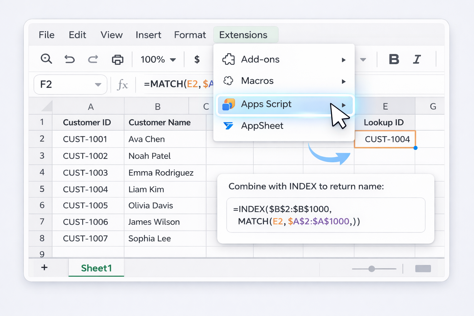
For recurring tasks—like matching weekly CSV exports to a master list—create a custom function in Apps Script that wraps MATCH.1. In Sheets, go to Extensions > Apps Script.2. Add a function: ```js function MATCH_ID(id, range) { return SpreadsheetApp.getActive() .getRange(range) .createTextFinder(id) .matchEntireCell(true) .findNext() .getRow(); } ```3. Use `=MATCH_ID(E2, "A2:A1000")` in your sheet.Pros: hides complexity from non‑technical users. Cons: requires light scripting to set up.**C. Power Query in Excel for fuzzy matching**When names or SKUs aren’t exact, MATCH alone struggles. Power Query can pre‑clean data.1. Select your table and go to Data > From Table/Range.2. Load both source and master tables into Power Query.3. Use Home > Merge Queries and enable “Use fuzzy matching”.4. Adjust similarity threshold and preview results.5. Load the merged output back to Excel, where MATCH/INDEX can work on the cleaned keys.Official docs:- Power Query overview: https://support.microsoft.com/en-us/excelPros: powerful for messy data. Cons: more steps, steeper learning curve for non‑analysts.### 3. Scaling MATCH with an AI agentAt some point, your challenge stops being “how do I write this one MATCH?” and becomes “how do I keep 50 workbooks and 200 MATCH-based reports accurate without my ops lead burning out?” This is where an AI computer agent like Simular becomes a force multiplier.**Method 1: Agent-driven spreadsheet building**You describe the outcome:- “Take this CRM export and this billing export, match on email, and build a cohort revenue report in Google Sheets.”The Simular agent:1. Opens your Sheets workbook.2. Inserts new tabs, pastes data from your exports.3. Writes appropriate MATCH/INDEX formulas, choosing match_type correctly and handling #N/A with IFERROR.4. Tests formulas on sample rows and adjusts ranges.Pros: non‑technical team members can get complex MATCH setups by describing them in plain language. Cons: you still need a clear data model and access permissions configured.**Method 2: Scheduled reconciliation across Excel and Sheets**For agencies and revenue teams, daily reconciliation is brutal. A Simular Pro agent can:1. Open your Excel finance workbook and Google Sheets CRM dashboard.2. Use MATCH to align invoice IDs, deal IDs, or subscription IDs across both tools.3. Color‑code mismatches, create summary sheets, and even email a brief.Because Simular is built as a general computer-use agent, it doesn’t just call APIs—it literally drives Excel and Google Sheets like a power user, but on autopilot.Pros: cross‑tool consistency, fewer manual checks. Cons: requires thoughtful onboarding (what sheets, what ranges, what counts as a mismatch).**Method 3: Massive backfills and data cleaning**When you inherit a chaotic stack of spreadsheets, an AI agent can:1. Iterate through folders on your drive.2. Open each Excel or Sheets file.3. Insert standardized MATCH-based checks (e.g., validate product IDs against a master catalog).4. Log failures into a central dashboard.Pros: turns a multi‑week clean‑up into an overnight job. Cons: you must review the first few runs carefully to ensure the matching rules and ranges are exactly what you intend.If you invest a couple of hours documenting how you currently use MATCH, you can then hand that "playbook" to an AI agent and let it scale your spreadsheet muscle across every workbook in your business.
Think of MATCH as the GPS and INDEX as the delivery driver. MATCH tells you *where* something is, INDEX fetches what lives there. This combo replaces many brittle VLOOKUPs.1) Set up your data: put lookup keys (like IDs or emails) in one column, and the value you want (price, owner, region) in a different column.2) Decide your lookup value. Example: customer ID in `E2`.3) In Excel or Google Sheets, find the position with MATCH: `=MATCH(E2,$A$2:$A$1000,0)` Use `0` for exact matches so order doesn’t matter.4) Wrap that inside INDEX to return the value from another column: `=INDEX($C$2:$C$1000, MATCH(E2,$A$2:$A$1000,0))` Here, `$C$2:$C$1000` is the column you actually want.5) Copy the formula down your sheet to apply it to many rows.This pattern works the same in Google Sheets and Excel, and is far more robust than VLOOKUP when columns move.
#N/A usually means MATCH couldn’t find what you asked for. That might be good (a new lead not in your CRM) or bad (a typo). Instead of hiding the error blindly, handle it deliberately.1) Wrap MATCH in IFERROR when you just need a clean fallback: `=IFERROR(MATCH(E2,$A$2:$A$1000,0),"")` This returns a blank when there’s no match.2) To debug, surface a message instead: `=IFERROR(MATCH(E2,$A$2:$A$1000,0),"Not found")`3) If you’re combining with INDEX, put IFERROR around the full expression: `=IFERROR(INDEX($C$2:$C$1000,MATCH(E2,$A$2:$A$1000,0)),"Check ID")`4) Check spaces and formatting. Use TRIM and UPPER/LOWER on both sides to normalize text.5) For Sheets, you can also use Data > Data cleanup tools to standardize input before matching.Handled well, #N/A becomes a signal that something new or broken has entered your pipeline—not a random annoyance.
Wildcards let MATCH work with partial or fuzzy text, which is perfect for messy business data: inconsistent company names, product variants, or people using different abbreviations.1) Use `*` for “any number of characters” and `?` for “one character”.2) Suppose `A2:A500` contains company names and you want the first one containing “Acme”. Use: `=MATCH("*Acme*",$A$2:$A$500,0)` The `0` forces an exact match on the *pattern*, not the full text.3) To match names that start with “Acme”, drop the leading star: `=MATCH("Acme*",$A$2:$A$500,0)`4) To match a SKU like “AB-1X3” where the middle character can vary, use: `=MATCH("AB-?X3",$A$2:$A$500,0)`5) If your data might literally contain * or ?, escape them with `~` (e.g., `"~*"`).Once MATCH finds the position, combine it with INDEX to pull all related fields—owner, segment, tier—so your team doesn’t need perfectly clean text to get useful results.
The `match_type` argument makes or breaks your results. The default (1) is dangerous if you don’t understand it.- `0` = exact match only. Use this for IDs, emails, SKUs—anything that should match perfectly. Order does not matter.- `1` = approximate, next *smaller* value. Use only when your lookup_array is sorted ascending (e.g., quantity thresholds). MATCH finds the largest value less than or equal to the lookup_value.- `-1` = approximate, next *larger* value. Use only when your lookup_array is sorted descending (e.g., risk scores where higher is riskier). MATCH finds the smallest value greater than or equal to the lookup_value.Best practice in business workbooks:1) Always specify `0`, `1`, or `-1` explicitly—never rely on the default.2) Add a comment near the formula explaining the sort order assumption.3) Consider wrapping approximate MATCH in IFERROR and test edge cases (values smaller than the minimum or larger than the maximum).This discipline prevents subtle, costly errors in pricing, commissions, or eligibility bands.
Once your operation depends on dozens of MATCH-driven reports—pipeline rollups, revenue reconciliations, channel attribution—maintenance becomes the real headache. Columns move, ranges grow, new sheets appear, and suddenly someone’s bonus relies on a broken formula.An AI agent like Simular can act as your spreadsheet operations assistant:1) Periodically open key Excel and Google Sheets workbooks.2) Scan for MATCH and INDEX+MATCH formulas and verify that named ranges and references still exist.3) Compare sample results against expected logic (e.g., a known customer ID should always return a specific region) and flag anomalies.4) Automatically extend ranges when new rows are added, or refactor formulas to use named ranges or structured tables.5) Log a changelog sheet describing what was checked and what was updated, so humans stay in control.This shifts your team from reactive firefighting—fixing broken MATCH formulas under deadline—to proactive monitoring, with an AI agent handling the tedious, error-prone checks at scale.