

If you run a sales team, agency, or online business, your Google Sheets are probably packed with messy text: lead sources, campaign names, tech stacks, job titles. The difference between a random list and a revenue engine is your ability to instantly see "who contains what"—who uses HubSpot, which rows mention "Demo requested", which contracts include a specific clause.
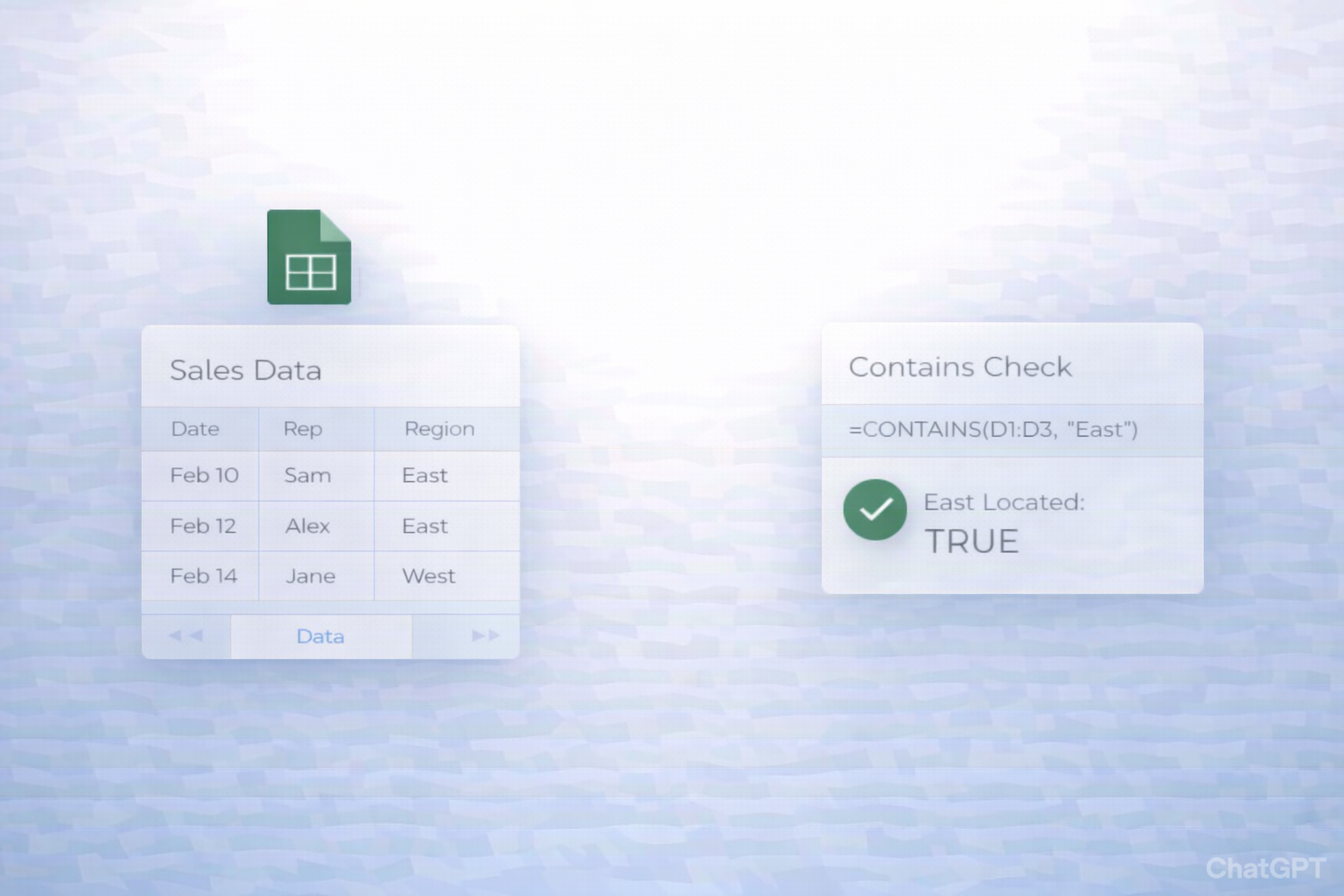
Because Google Sheets has no native IF CONTAINS function, the real power comes from combining IF, REGEXMATCH, SEARCH, and COUNTIF to replicate SQL-style contains logic. You can tag rows, route leads, and trigger follow-ups with a single formula. But doing this across tens of tabs and constantly changing data quickly becomes a grind.This is where delegation to an AI computer agent changes the game. Instead of you hunting for text patterns every morning, the agent opens Sheets like a human, applies contains rules, updates tags, and even kicks off downstream workflows. You get clean, classified data and always-on monitoring without burning your team’s focus on low-leverage spreadsheet work.
## 1. Manual ways to use "contains" in Google SheetsBefore you scale, you need solid basics. Here are core manual techniques your team should know.### 1.1 IF + REGEXMATCH: the classic "IF CONTAINS"This combo recreates a SQL-style IF CONTAINS.**Use case:** Tag leads whose tech stack contains "G Suite".Formula:`=IF(REGEXMATCH(D2, "G Suite"), "Uses G Suite", "No")`**Steps:**1. In a new column (e.g., E2), paste the formula above.2. Replace `D2` with the cell that holds your text and `"G Suite"` with your keyword.3. Drag the fill handle down the column to apply it to all rows.4. Filter on the new column to see only rows that match.Docs:- IF: https://support.google.com/docs/answer/3093364- REGEXMATCH: https://support.google.com/docs/answer/3098242### 1.2 REGEXMATCH alone for TRUE/FALSE flagsSometimes you just need a boolean you can combine with other logic.Formula:`=REGEXMATCH(B2, "HubSpot")`Returns TRUE if B2 contains "HubSpot", FALSE otherwise. Great for building layered conditions like:`=IF(AND(REGEXMATCH(B2, "HubSpot"), REGEXMATCH(C2, "G Suite")), "High-fit", "Other")`### 1.3 SEARCH + ISNUMBERAnother way, closer to Excel’s style, is `SEARCH` wrapped in `ISNUMBER`.Formula:`=ISNUMBER(SEARCH("Tolkien", A2))`**Steps:**1. `SEARCH("Tolkien", A2)` returns the character position of the match or an error.2. `ISNUMBER(...)` converts that into TRUE/FALSE.Docs:- SEARCH: https://support.google.com/docs/answer/3093378- ISNUMBER: https://support.google.com/docs/answer/3093321### 1.4 COUNTIF for "contains and count"When you want to know *how many* cells contain a phrase:Formula:`=COUNTIF(D:D, "*G Suite*")`The asterisks are wildcards, meaning "anything before or after".Docs:- COUNTIF: https://support.google.com/docs/answer/3093480### 1.5 Filter views with "Text contains"For quick visual analysis:1. Select your header row.2. Go to **Data → Create a filter**.3. Click the filter icon on a column.4. Choose **Filter by condition → Text contains** and type your keyword.This is ideal for fast, ad-hoc exploration by sales and marketing teams.---## 2. No‑code automation: make "contains" run itselfManual formulas are powerful, but they still rely on humans opening the sheet. Let’s move toward automation with low/no-code tools.### 2.1 On‑edit highlighting with conditional formattingYou can visually flag cells that contain certain text the moment someone types it.1. Select the range (e.g., `A2:A1000`).2. Go to **Format → Conditional formatting**.3. Under **Format cells if**, choose **Text contains**.4. Enter your keyword (e.g., "Hot lead").5. Pick a bold fill color and click **Done**.Now any time your team enters that phrase, the cell auto-highlights—no extra work.Docs:- Conditional formatting: https://support.google.com/docs/answer/78413### 2.2 Use IF + REGEXMATCH as a reusable "rule column"Turn contains logic into a standard rule column everyone relies on.1. Create a dedicated "Routing rule" or "Segment" column.2. Insert a formula like: `=IFS( REGEXMATCH(B2, "demo"), "Demo requested", REGEXMATCH(B2, "refund|cancel"), "Churn risk", TRUE, "Other" )`3. Drag down the column.4. Train your team to filter, pivot, and report from this rule column only.This keeps logic centralized and easy to adjust as messaging and campaigns evolve.Docs:- IFS: https://support.google.com/docs/answer/7014145### 2.3 Connect to workflow tools (Zapier/Make) without codeWhile not official Google tools, platforms like Zapier or Make let non-technical teams automate around Google Sheets.**Example: Alert sales when a row "contains" buying intent.**1. In Sheets, add a column with: `=REGEXMATCH(C2, "book a call|demo")`.2. In Zapier, set a trigger: "New or updated row in Google Sheets".3. Add a filter step: proceed only if the column is TRUE.4. Action: send a Slack message or email to the account owner with row details.Now every time a prospect types buying language, your team hears about it instantly—no one needs to patrol the sheet.Official Sheets API/automation overview:- https://developers.google.com/sheets/api---## 3. Scaling "contains" with AI computer agentsAt some point, even no-code automations hit limits. You end up with dozens of sheets, edge cases, and tools that don’t talk cleanly. This is where a Simular AI agent becomes your tireless operations assistant.Simular Pro (https://www.simular.ai/simular-pro) is a highly capable AI computer agent that can operate across your desktop, browser, and cloud apps just like a human—clicking, typing, filtering, copying, pasting—only 24/7 and without context fatigue.### 3.1 Agent-driven lead and account classification**Story:** Imagine your agency pulls company lists from tools like Koala, LinkedIn, and exports from CRMs. You want to know which rows in Google Sheets contain certain tech stack keywords ("HubSpot", "G Suite", "Shopify") and route them to specialists.**How Simular handles it:**1. The agent opens your lead sheet in Google Sheets.2. It inserts or updates formulas like `=IF(REGEXMATCH(D2, "G Suite"), "G Suite", "-")` across thousands of rows.3. It applies filters and sorts to group targets by stack.4. It copies high-fit accounts into a "Priority" sheet and logs summary stats in a recap tab.5. Via webhook integration, it can notify Slack or update your CRM.**Pros:**- Works across tools without brittle APIs.- Fully transparent: every step is visible and editable.- Handles huge, evolving sheets and complex rules.**Cons:**- Best for recurring, structured workflows (not one-off tiny tasks).- Requires a short upfront definition of the workflow.### 3.2 Continuous monitoring and reporting**Story:** A growth lead wants a daily rollup: "How many rows contain ‘trial’, ‘cancel’, or ‘upgrade’ across multiple feedback and support sheets?"**With Simular:**1. On a schedule, the agent opens each relevant Google Sheet.2. It uses a mix of COUNTIF and REGEXMATCH-based helper columns to compute daily counts.3. It updates a master dashboard sheet and optionally transforms results into a Google Doc or email brief.You’ve effectively turned vague text into quantified signals without a human ever touching the formulas.**Pros:**- Handles multi-sheet, multi-source logic.- Turns free-form text into consistent, daily metrics.**Cons:**- Overkill if you only maintain one small sheet.### 3.3 Complex cross-app workflowsBecause Simular can automate "nearly everything a human can do" on a computer, you can chain Google Sheets contains logic into full revenue workflows:- Scan a sheet for rows where notes contain "ready to buy".- Open your CRM in the browser.- Update opportunity stages and owners.- Draft personalized outreach based on context, ready for human review.With production-grade reliability and transparent execution, you’re not trusting a black box—you’re giving a very fast, very precise assistant the keyboard and mouse while you focus on strategy.
To check if a cell includes specific text in Google Sheets, combine IF with REGEXMATCH. This mimics a true IF CONTAINS. Suppose column B holds comments and you want to tag any row that mentions "demo".Use this formula in C2:`=IF(REGEXMATCH(B2, "demo"), "Mentions demo", "No demo")`Explanation:- `REGEXMATCH(B2, "demo")` returns TRUE if "demo" appears anywhere in B2, regardless of position.- IF then returns the label you choose for TRUE or FALSE.Steps:1. Insert a new column for your tag.2. Paste the formula in the first data row.3. Drag the formula down to apply it to all rows.4. Use **Data → Create a filter** and filter on your tag column to work only with matches.Docs: IF (https://support.google.com/docs/answer/3093364), REGEXMATCH (https://support.google.com/docs/answer/3098242).
To count how many cells contain certain text, use COUNTIF with wildcards. Wildcards `*` mean "any characters before or after" your search term.Example: count how many entries in D2:D500 mention "G Suite" anywhere in the cell.Formula:`=COUNTIF(D2:D500, "*G Suite*")`Explanation:- `D2:D500` is the range to scan.- `"*G Suite*"` tells Sheets: match any text that has "G Suite" inside it.Steps:1. Decide the range you want to analyze (e.g., a column of tech stacks).2. In a summary cell, enter the COUNTIF formula with your range and pattern.3. Adjust the keyword and range as needed for other metrics, such as `"*HubSpot*"` or `"*cancel*"`.4. Build a small metrics table with multiple COUNTIF rows to track several keywords at once.Docs: COUNTIF (https://support.google.com/docs/answer/3093480).
To apply contains logic across an entire column in Google Sheets, create a helper column with a formula in the first data row, then fill it down. For example, if A contains email subject lines and you want to flag those that reference "refund" or "cancel", do this:1. Add a new column header, e.g., "Churn intent" in B1.2. In B2, enter:`=IF(REGEXMATCH(A2, "refund|cancel"), "Churn signal", "-")`3. Hover over the bottom-right corner of B2 until you see the fill handle, then double-click it. Sheets auto-fills the formula down to the last contiguous row.4. Filter, group, or pivot using the new "Churn intent" column.This pattern scales nicely: keep your raw text in one column and your normalized, contains-based classification in another. When new rows are added in the middle, check that the formula has extended; if not, re-fill it down.
By default, REGEXMATCH in Google Sheets is case-sensitive, but you can make checks case-insensitive by using LOWER on both the text and the search term. This is useful when user-entered data might be "Demo", "demo", or "DEMO".Example: flag rows where column C mentions "vip" in any capitalization.Formula in D2:`=IF(REGEXMATCH(LOWER(C2), "vip"), "VIP", "")`Explanation:- `LOWER(C2)` converts the entire cell to lowercase.- `REGEXMATCH(LOWER(C2), "vip")` now only needs a lowercase pattern.Steps:1. Decide which column holds the free-text values.2. Insert a helper column for the case-insensitive flag.3. Use the LOWER + REGEXMATCH combo as above.4. Drag down to cover all rows.You can also use this approach inside more complex formulas, such as IFS, to build robust, case-insensitive segmentation rules that survive messy, real-world data.
An AI computer agent like Simular can take your Google Sheets contains logic and run it at scale, hands-free. Instead of you opening a sheet, writing formulas, and checking results, the agent behaves like a power user on autopilot.A typical workflow:1. You define the rules: which columns to scan, which phrases matter (e.g., "demo", "cancel", "G Suite"), and what tags or actions each should trigger.2. Simular opens your Sheets in the browser or desktop app.3. It inserts or updates helper columns with formulas like `=IF(REGEXMATCH(D2, "G Suite"), "G Suite", "-")`.4. It applies filters, builds summaries with COUNTIF, and copies high-value rows into a separate tab or report.5. Through webhooks, it can then update a CRM, notify Slack, or launch follow-up tasks.Because every action is transparent and inspectable, you can see and refine exactly how the agent uses contains logic while reclaiming hours of manual spreadsheet work.