How To Master XLOOKUP in Google Sheets: A Smart Guide

If your day starts with coffee and a Google Sheets tab, XLOOKUP is probably one of your best friends—or your next big unlock. Let’s walk through how to use it manually, then how to scale the same logic with an AI computer agent so you never have to babysit formulas again.

‍

1. The Classic Manual Way: Exact Match XLOOKUP

Goal: Look up a value (like a client ID) and return a related value (like MRR).

Step-by-step:

1. Organize your data so the key you want to search is in one column (the lookup range) and the result you want is in another (the result range).
2. Click into the cell where you want the result.
3. Type a basic formula, for example: =XLOOKUP(A2, Sheet2!A2:A1000, Sheet2!C2:C1000)
   • A2 is your search_key (e.g., client ID).
   • Sheet2!A2:A1000 is the lookup_range.
   • Sheet2!C2:C1000 is the result_range.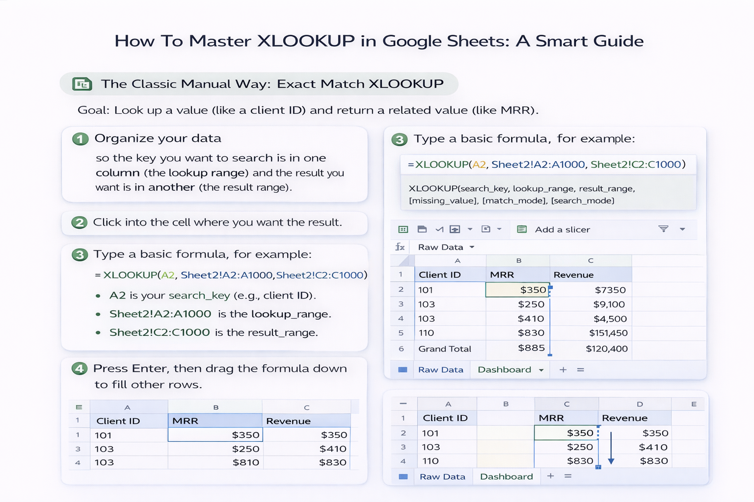
4. Press Enter, then drag the formula down to fill other rows.

Pros: Simple, transparent, great for small to medium data. ‍

‍Cons: Easy to break when ranges change; copying formulas across thousands of rows is tedious.

‍

2. Handling Missing Values and Cleaner Dashboards

XLOOKUP can gracefully handle missing data so your dashboards don’t shout #N/A at every corner.

Example: =XLOOKUP(A2, Sheet2!A:A, Sheet2!C:C, "Not Found")

Here, the fourth argument is the missing_value. Instead of an error, you get a friendly label you can filter on.

Use this pattern when:

• Your sales or CRM export is incomplete.
• Product IDs may not yet exist in the pricing sheet.
• You’re matching leads from multiple campaigns.

Pros: Cleaner reporting and fewer support pings about “broken” sheets.

‍Cons: Still manual; you’re responsible for every new column, every new tab, every new data dump.

‍

3. Cross-Sheet and Horizontal Lookups

Real businesses rarely keep everything on one tab. XLOOKUP thrives when your data is spread across different sheets.

Cross-sheet example: =XLOOKUP(A2, Metrics!A:A, Metrics!D:D)

Horizontal example: =XLOOKUP("Q4", B1:Z1, B2:Z2)

You can:

• Pull the right commission rate based on territory.
• Match a client to the current plan tier.
• Fetch a quarterly target from a wide timeline table.

Pros: Flexible layout; no need to reorder tables.

‍Cons: As the workbook grows, so does the cognitive load of tracking where everything lives.

‍

4. Multi-Criteria Lookups With XLOOKUP

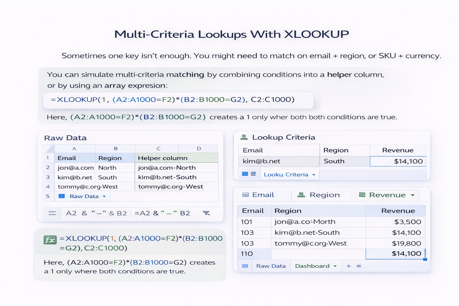
Sometimes one key isn’t enough. You might need to match on email + region, or SKU + currency.

You can simulate multi-criteria matching by combining conditions into a helper column, or by using an array expression:

=XLOOKUP(1, (A2:A1000=F2)*(B2:B1000=G2), C2:C1000)

Here, (A2:A1000=F2)*(B2:B1000=G2) creates a 1 only where both conditions are true.

Pros: Powerful, avoids tangled INDEX/MATCH stacks.

‍Cons: Easy to mis-type, hard for non-technical teammates to maintain.

‍

5. Where Manual XLOOKUP Breaks Down

Manual XLOOKUP is fine when:

• You have one or two source sheets.
• Schema changes are rare.
• Only one or two spreadsheet-savvy people touch the file.

It breaks down when:

• You’re reconciling exports from CRM, billing, and ad platforms daily.
• Your team constantly adds new columns or tabs.
• You copy similar XLOOKUP setups across dozens of clients.

This is exactly where an AI computer agent shines.

‍

6. Scaling XLOOKUP With an AI Computer Agent

Instead of you hopping between tabs, an AI agent running on your desktop can:

• Open Google Sheets in the browser.
• Understand which column is the lookup key and which is the result.
• Write the appropriate XLOOKUP formula for each sheet.
• Drag-fill formulas down thousands of rows.
• Adjust ranges when new rows or columns are added.

You describe the intent once: “Match customer_id in this sheet to the MRR column in that sheet and populate MRR in column G.” The agent does the clicking, typing, and verifying.

Pros:

• Massive time savings for recurring reporting.
• Fewer broken formulas when structures change.
• Non-technical teammates can request changes in plain language.

Cons:

• Requires an initial setup and onboarding of the agent.
• You still need to define good data structure and naming.

‍

7. Hybrid Workflow: You Design, the Agent Maintains

The sweet spot for most knowledge workers is hybrid:

• You design the first version of the model and key XLOOKUP patterns so logic matches the business.
• The agent applies, maintains, and scales that logic across files, clients, and weeks of new data.

Over time, you stop being the “spreadsheet person” everyone Slacks at 10 p.m. The agent becomes the one who extends ranges, rewires formulas after a column is inserted, and keeps your Google Sheets XLOOKUP universe humming while you focus on strategy, not syntax.