

If you run a sales team, an agency, or a growing ecommerce brand, you probably live in Google Sheets. Revenue by month, campaign performance by channel, SKU pricing across regions — all neatly arranged in rows with dates or IDs on top. HLOOKUP is the quiet hero here: it scans that first row for a key (like a month, product ID, or plan tier) and instantly pulls the matching value from any row beneath. Once you understand search_key, range, index, and the is_sorted flag, you can turn messy horizontal logs into reliable, reusable dashboards. No more manual hunting through columns or copy‑pasting numbers into client reports. HLOOKUP makes your top row the control panel for the rest of the sheet. Now imagine you no longer even touch those formulas. An AI computer agent opens Google Sheets, builds the HLOOKUP formulas, fixes #N/A errors, and updates ranges after every new campaign. It becomes your invisible ops analyst, quietly running the same lookup logic across dozens of sheets while you stay focused on deals, strategy, and clients.
HLOOKUP is one of those functions that feels trivial until you need it across 20 client sheets, 12 months of data, and a fast‑moving sales team. Let’s walk through how to use it well, then how to automate it so you never have to explain it twice.## 1. Manual ways to use HLOOKUP in Google Sheets### 1.1 Understand the core syntaxBefore anything else, lock in the basics. The official Google help page is here: https://support.google.com/docs/answer/3093375?hl=enThe syntax: =HLOOKUP(search_key, range, index, [is_sorted])• search_key: what you’re looking for in the first row (like a month name or product ID).• range: the full table, including the header row and all rows you might return.• index: which row (within that range) you want back, where the first row is 1.• is_sorted: FALSE for exact match (recommended for business data), TRUE for approximate.### 1.2 Build a simple revenue by month lookup
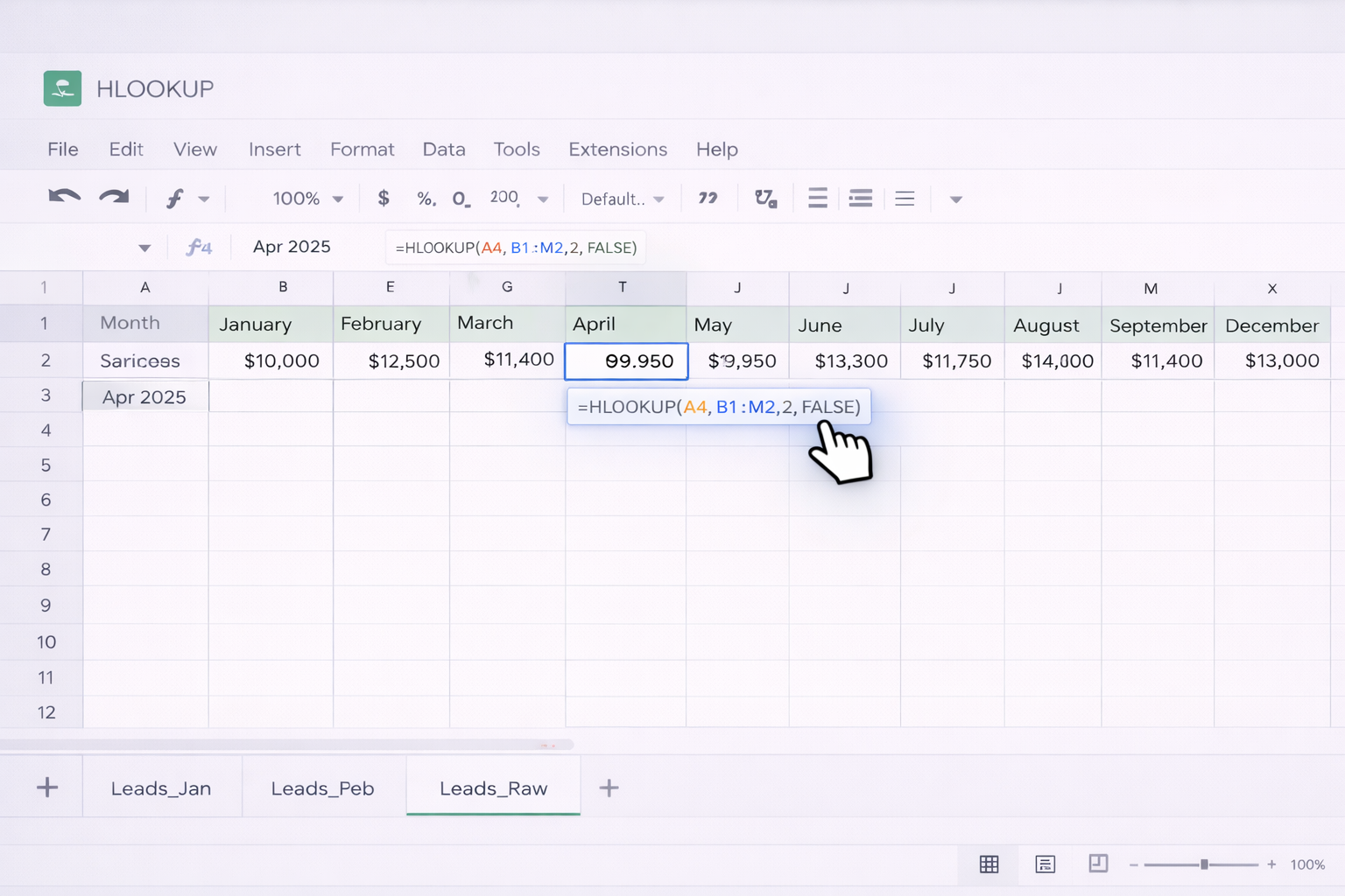
Scenario: You have months across row 1 (B1:M1) and total revenue for each month in row 2.1) Click the cell where you want the result, e.g. B4.2) Type: =HLOOKUP(A4, B1:M2, 2, FALSE) • A4 holds the month you’re querying (e.g. 'Apr 2025'). • B1:M2 is your header plus revenue row. • 2 tells Sheets to return data from the second row of that range (the revenue). • FALSE forces an exact match so a typo becomes an obvious #N/A error.3) Test by changing A4 to other months. The result should update instantly.### 1.3 Product pricing table for sales teamsImagine SKUs across row 1, and different price tiers in rows 2–4.1) Put SKUs in row 1 (B1:F1), and rows 2–4 as 'List', 'Partner', 'Promo' pricing.2) In a quote sheet, let B3 hold the SKU, and C3 hold the price tier label.3) Create a mapping row index (e.g. row 6) where you convert the tier label to the correct index (1 for list, 2 for partner, etc.), maybe via IF or SWITCH.4) Use: =HLOOKUP(B3, Pricing!B1:F4, Pricing!B6, FALSE)This lets your team type a SKU and tier and instantly get the right number.### 1.4 Avoid common HLOOKUP errorsFrom the docs and real‑world use:• If index is less than 1 or more than the number of rows in range, you’ll see #VALUE! Fix by checking your range and index.• If the search_key isn’t in the first row, you’ll get #N/A. Either fix your header or adjust the range.• If you use TRUE for is_sorted but the header row isn’t sorted, you may get wrong values. For business logic, default to FALSE unless you truly need approximate matches.### 1.5 Handle duplicate headers carefullyWhen the same header appears twice (for example, a client that launched two separate campaigns in the same month), HLOOKUP returns the first occurrence only. Best practice:• Make your header keys unique (e.g. 'Apr 2025 – Brand', 'Apr 2025 – Performance').• Or use a different structure (VLOOKUP or FILTER) when duplicates are unavoidable.## 2. No‑code automation around HLOOKUPOnce your formulas work, the next bottleneck is feeding them fresh data and keeping ranges in sync. No‑code tools can pipe data into Google Sheets so HLOOKUP always points at a living table instead of a static export.### 2.1 Use Google Apps Script for dynamic ranges
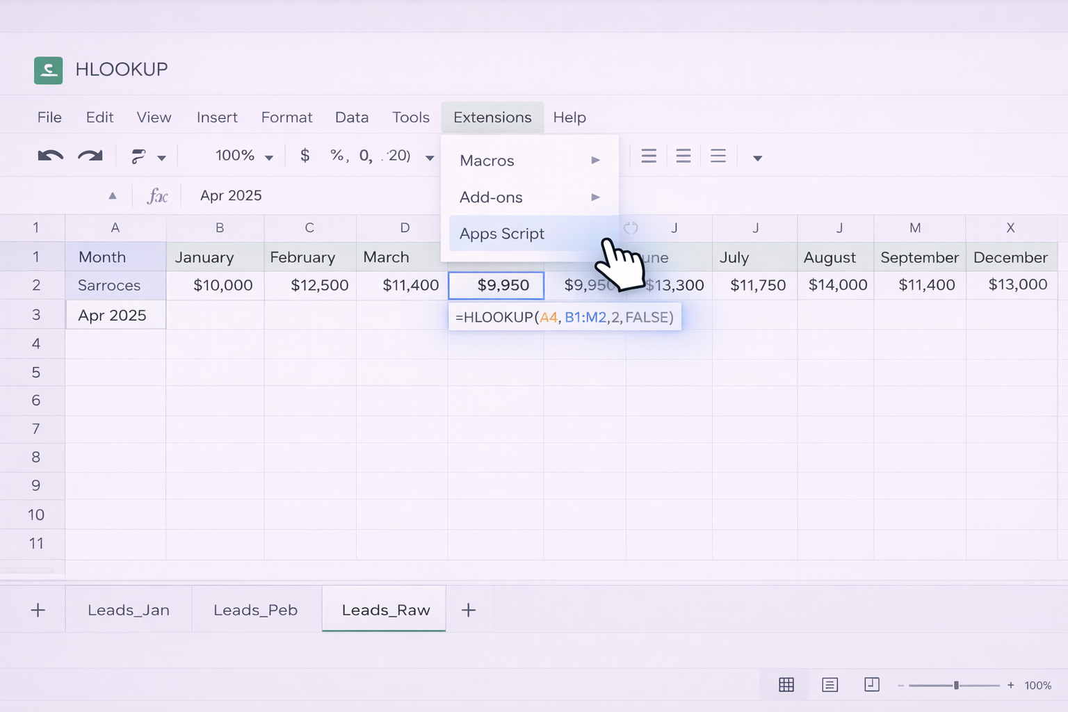
You can use simple Apps Script to update the range that HLOOKUP references when new columns are added.1) In Sheets, go to Extensions → Apps Script.2) Add a script that uses getLastColumn() to find the latest column in your dataset.3) Build a named range programmatically (e.g. 'RevenueTable') and update it whenever the sheet changes.4) Point HLOOKUP at the named range instead of a fixed B1:M2.Official Apps Script docs: https://developers.google.com/apps-script/guides/sheets### 2.2 Connect external data with no‑code toolsTools like Zapier or Make can push CRM, ad, or ecommerce data into Sheets on a schedule.A typical sales workflow:1) Trigger: 'New deal won' in your CRM.2) Action: Append deal details into a 'Won Deals' sheet with months along the top row.3) Your summary sheet uses HLOOKUP to pull monthly totals, average deal size, or channel‑specific metrics into dashboards.4) When a new month appears, the automation adds a new column, and your HLOOKUP (if using a dynamic range or named range) sees it immediately.This keeps your finance, revenue ops, and account teams aligned without anyone exporting CSVs.### 2.3 Validate data before HLOOKUP runsUse Data → Data validation in Sheets to restrict header values to a known list (e.g. months, SKUs). This dramatically reduces #N/A caused by typos and keeps automations stable.## 3. Scaling HLOOKUP with an AI agentManual and no‑code approaches still assume a human is checking formulas and fixing edge cases. An AI computer agent like Simular’s desktop‑level agent can go further by actually operating Google Sheets on your behalf.### 3.1 Let an AI agent build and audit HLOOKUP logicA Simular AI agent can:• Open your Google Sheets dashboard in the browser.• Read your business context from a brief (for example, which rows hold revenue, which hold cost, which hold targets).• Insert correct HLOOKUP formulas in target cells, using exact‑match FALSE, correct index values, and named ranges.• Cross‑check results by spot‑calculating a few values and comparing them to expectations.Pros: Removes formula anxiety for non‑technical team members; ensures consistent patterns across many files.Cons: Requires an initial, well‑designed prompt and access setup for the agent.### 3.2 Automate cross‑sheet reporting at scaleImagine 30 client folders, each with its own performance log sheet.The Simular AI agent can:1) Iterate through a list of Google Sheets URLs in a control sheet.2) For each sheet, identify the header row and confirm it matches your standard.3) Insert or update HLOOKUP formulas in a master report sheet that pulls KPIs (CPA, ROAS, revenue) from every client file.4) Log successes and any anomalies into a 'QA' sheet you can quickly review.Pros: Scales your reporting without hiring more analysts; every new client gets the same, proven structure.Cons: The first run takes careful testing, and you’ll want transparent execution logs (something Simular Pro is designed to provide) so you can inspect each step.### 3.3 Self‑healing spreadsheetsBecause Simular’s agents can run thousands to millions of actions reliably, you can schedule them to:• Open critical dashboards daily.• Scan for #N/A, #VALUE!, or #REF! in key HLOOKUP cells.• Diagnose whether the cause is a missing header, changed range, or incorrect index.• Apply fixes, update named ranges, or flag issues that truly need human input.Over time, your sheets become living systems instead of fragile one‑off models. You stay focused on strategy, while the AI quietly does the clicking, checking, and formula surgery in the background.
Start with a simple, controlled example. First, arrange your data so that the values you want to search by (months, product IDs, plan names) are in the first row of a range, with the data you want to return in rows below. For example, put months in B1:M1 and corresponding revenue in B2:M2. Then choose a cell for your result, say B4, and type: =HLOOKUP(A4, B1:M2, 2, FALSE). In this setup, A4 holds the month you want to look up (e.g. 'Apr 2025'), B1:M2 is the table, 2 tells HLOOKUP to return the second row (revenue), and FALSE enforces an exact match. Press Enter and confirm the correct number appears. Test by changing A4 to other months. If you see #N/A, check for typos in the search key or whether that column actually exists in the header row.
#N/A means HLOOKUP cannot find the search_key in the first row of the specified range. To fix it, walk through these checks: 1) Confirm your header row is included in the range and is the very first row of that range. If your months are in row 3, your range should start at row 3, not row 4. 2) Make sure your search_key is spelled and formatted exactly like the header (dates in particular must be real dates, not text). 3) If you used FALSE as the last argument, HLOOKUP requires an exact match; if the key simply doesn’t exist, #N/A is correct. Add the missing column or adjust your expectations. 4) If you used TRUE, ensure the header row is sorted ascending; otherwise HLOOKUP might stop in the wrong place. For business data, default to FALSE and use data validation on the search cell to prevent typos.
Index in HLOOKUP tells Sheets which row within your range to return. The first row of the range is 1, the next is 2, and so on. Many errors come from miscounting this. To get it right, first highlight your range and mentally label each row inside it. For example, if your range is B1:B4, then row B1 is index 1, B2 is 2, B3 is 3, B4 is 4. If revenue is in B2 and profit in B3, use index 2 for revenue and 3 for profit. When your table grows, consider freezing a helper column with index numbers listed down the side (1,2,3,4) aligned with each row; that makes it obvious which index to use. If you insert a new row into the middle, remember indexes will shift; this is where named ranges or an AI agent that auto‑audits your formulas can prevent silent misalignment.
Yes, but you must be deliberate with the is_sorted parameter. When your header row is not strictly sorted (for example, custom month order, SKUs mixed with special labels), always set the last argument of HLOOKUP to FALSE. This tells Sheets to search for an exact match only and avoids the approximate‑match behavior that can return wrong values on unsorted data. For example: =HLOOKUP('SKU‑123', A1:Z5, 3, FALSE). If you leave is_sorted blank or set it to TRUE, Sheets assumes the first row is sorted ascending and will perform a binary search; with unsorted data it may stop early and return an incorrect value without an obvious error. For financial or performance reporting, default to FALSE and rely on #N/A as a signal that your header or input is wrong, not a silent guess.
To automate HLOOKUP across dozens of Google Sheets, combine structure, naming, and automation. First, standardize each sheet: use the same header row labels and keep key metrics in consistent rows so a single HLOOKUP pattern works everywhere. Next, build a master control sheet that lists the URLs or IDs of each client or department sheet. Manually, you can use IMPORTRANGE plus HLOOKUP to pull values, but this quickly becomes hard to maintain. A better approach is to use Apps Script or an AI computer agent. With Apps Script, loop through the control list, open each sheet programmatically, and write HLOOKUP formulas into a central report. With an AI agent like Simular, you can literally have the agent open each file in the browser, confirm headers, insert or fix formulas, and log any anomalies. This combination lets non‑technical teams get consistent, up‑to‑date metrics without ever touching the formulas themselves.