
Oops! Something went wrong while submitting the form.
.svg)
VLOOKUP is the quiet workhorse behind most business spreadsheets. In Google Sheets, it lets you pull prices, owner names, campaign tags, or CRM IDs from a single source of truth into the sheet where decisions actually happen. Instead of retyping data or trusting your memory, you give Sheets a search key—an email, SKU, or employee ID—and it returns the matching details from another column or even another tab. For agencies, sales teams, and operators, this means cleaner reports, faster forecasts, and fewer “where did this number come from?” moments. As those sheets grow, though, maintaining hundreds of VLOOKUPs becomes a job in itself. Delegating that maintenance to an AI computer agent means the agent can insert and copy formulas, switch ranges when a dataset moves, and troubleshoot #N/A errors at scale. You stay focused on strategy; the agent handles the grunt work of keeping every lookup fast, accurate, and up to date.
Every business has a “spreadsheet person” — the one everyone pings when a report breaks or a VLOOKUP stops working. If that person is you, there’s good news: you can teach both humans and AI agents to share the load.
Before automating anything, it’s crucial to understand what “correct” looks like.
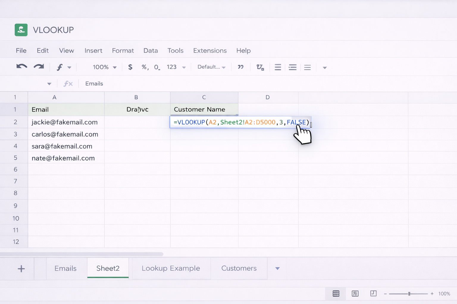
D2.=VLOOKUP(search_key, range, index, FALSE)
search_keyA2.rangeSheet2!A2:D5000.indexindex = 3.is_sortedFALSE for an exact match: ...,3,FALSE).Pros (manual):
Cons (manual):
Real-world data rarely lives in one neat table.
=VLOOKUP(A2,Products!$A$2:$D$500,3,FALSE)
$ to drag safely.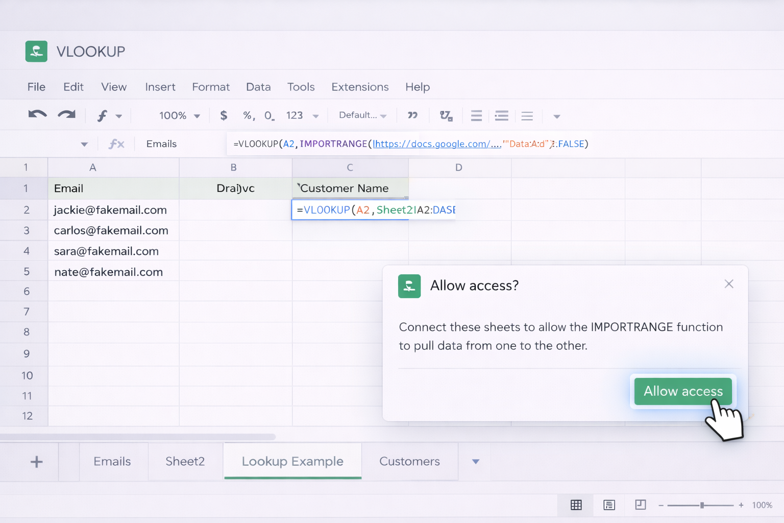
IMPORTRANGE:=IMPORTRANGE("https://docs.google.com/...", "Data!A2:D")
=VLOOKUP(A2,IMPORTRANGE("url","Data!A2:D"),3,FALSE)
Pros (cross-sheet):
Cons (cross-sheet):
Imagine an assistant who never tires of:
Simular Pro works like a human on your desktop and browser:
Pros (AI-powered):
Cons (AI-powered):
Manual VLOOKUP is fine for a small spreadsheet once a month. Consider automation if you:
Rule of thumb: you define the rules; the agent does the clicking, typing, and checking at scale. You focus on insights, strategy, and telling the story the numbers reveal.
