
.svg)
.svg)
.svg)
Every business has a version of the same story: a “simple” Google Sheets report that behaves strangely. Totals don’t add up, filters feel off, and your gut says something’s wrong. Often the culprit is hidden text-formatted numbers—values that look like 1200, but behave like the word “twelve hundred.”
Learning how to reliably convert text to numbers in Google Sheets is about more than spreadsheet hygiene. It protects your revenue forecasts, ad performance reports, sales pipelines, and client dashboards from silent errors. Once you understand the manual methods—VALUE(), formatting, ARRAYFORMULA, and regex—you can debug almost any messy import.
But for agencies, operators, and growth teams, doing this cleanup by hand on every CSV import is a tax on your best people. That’s where an AI agent comes in. An AI computer agent can watch for new data, open the right Google Sheets, run conversion formulas across thousands of rows, validate with ISNUMBER checks, and log what changed. You go from babysitting spreadsheets to simply reviewing clean, trustworthy numbers at the end of each run.
You’ve just imported a chunky CSV from your CRM or ad platform into Google Sheets. Everything looks fine—until your SUM formula returns zero. The numbers aren’t really numbers. They’re text.
Let’s walk through the best ways to fix this manually, then scale it with an AI computer agent so you never fight this battle twice.
This is the first thing to try when values look like numbers but behave like text.
Steps:
Pros:
Cons:
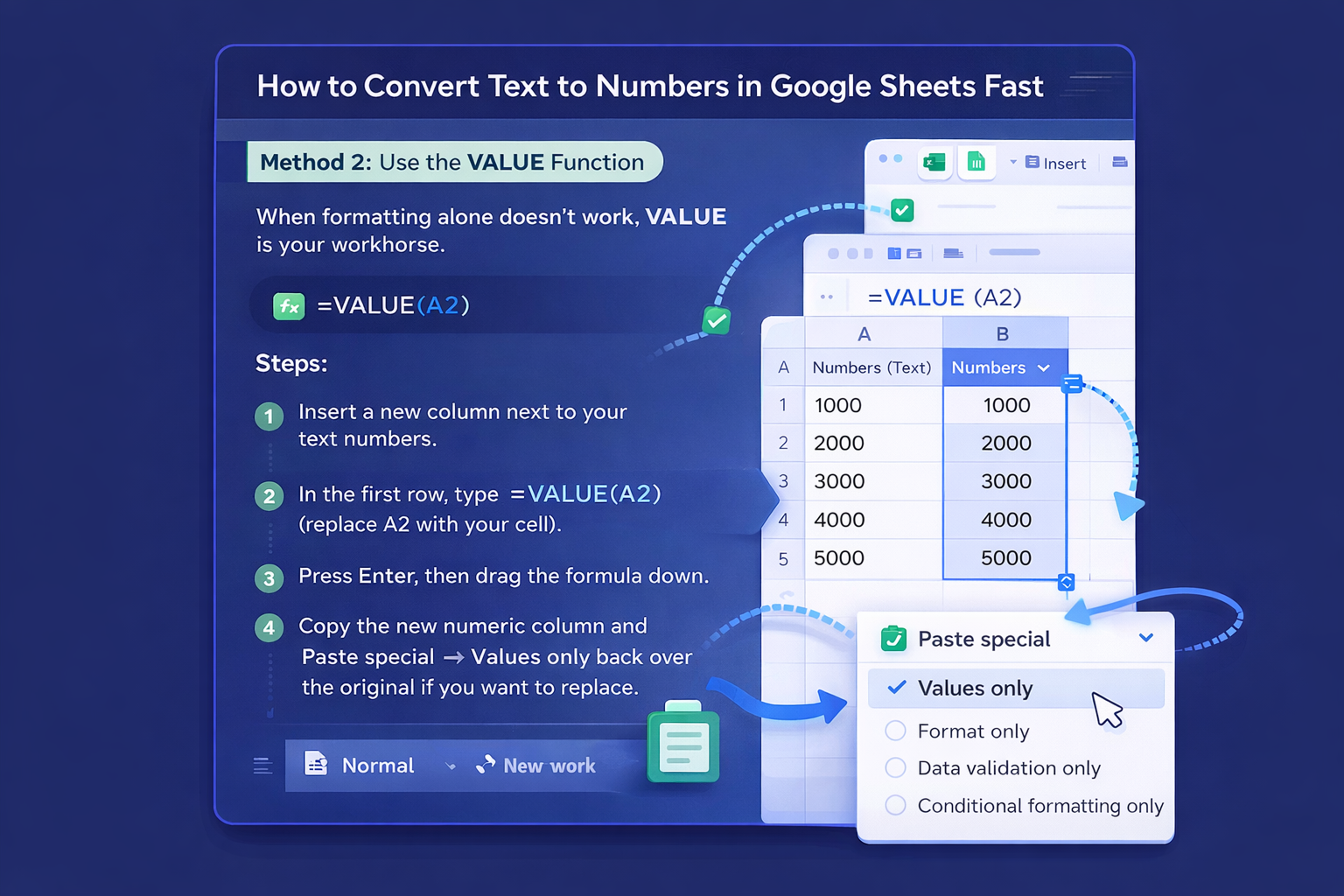
When formatting alone doesn’t work, VALUE is your workhorse.
Formula: =VALUE(A2)
Steps:
=VALUE(A2) (replace A2 with your cell).
Pros:
Cons:
$, labels, or stray text.
This is the classic “brute force” trick.
Formula: =A2*1
Steps:
=A2*1 in the first helper cell.
Pros:
Cons:
Real business data is rarely clean. Think "Price: $199" or "Revenue (EUR) 1,234.50". For that, you need slightly sharper tools.
Formula example: =VALUE(REGEXREPLACE(A2, "[^\d.]", ""))
What it does:
REGEXREPLACE strips everything except digits and decimal points.VALUE converts the cleaned string into a number.
Steps:

Pros:
Cons:
If you’re converting hundreds or thousands of rows, ARRAYFORMULA saves you from dragging formulas.
Basic example: =ARRAYFORMULA(VALUE(A2:A))
Steps:
Pros:
Cons:
Never trust a conversion until you verify it.
Formula: =ISNUMBER(B2)
Steps:
=ISNUMBER(your_converted_cell).This tiny check can save a campaign report, a revenue forecast, or a client relationship.
Manual fixes are fine the first time. They’re a problem the tenth time.
Imagine an AI computer agent that:
That’s where a production-grade agent platform like Simular comes in. Instead of relying on one-off scripts, you spin up a computer-use agent that behaves like a meticulous analyst: clicking, selecting ranges, typing formulas, inspecting cells, and retrying if something fails.
Set up once, test it on a few messy spreadsheets, then let the agent take over. Your future self—and your future dashboards—will thank you.
If your “numbers” in Google Sheets sort as 1, 100, 12 instead of 1, 12, 100, they’re stored as text. Check alignment first: text is usually left-aligned. Then try changing the format to Number or using =VALUE(A2) in a helper column, filling it down, and pasting values back to convert everything to real numeric data.
To convert a whole column, use ARRAYFORMULA with VALUE. In an empty column, enter =ARRAYFORMULA(VALUE(A2:A)). This applies VALUE down the entire range automatically. Review the results, then copy the converted column and use Paste special → Values only to replace the original text column if everything looks correct.
When cells contain labels or symbols like “Price: $99.99”, combine REGEXREPLACE with VALUE. Use =VALUE(REGEXREPLACE(A2, "[^\d.]", "")) to strip everything except digits and decimal points, then convert the result. Test the formula on a few rows, ensure the numbers match expectations, and then apply it down the entire column.
Imported CSVs often store numbers as text. First, try Format → Number. If that fails, add a helper column with =VALUE(A2) or =A2*1. For messy strings, use REGEXREPLACE to remove extra characters. Once the numbers look right, convert the entire helper column to values and delete or hide the original text-based column.
You can automate by combining formulas with an AI computer agent. Define a repeatable playbook: detect new data, apply VALUE or ARRAYFORMULA, use REGEXREPLACE for mixed strings, and validate via ISNUMBER. A Simular-style agent can execute this flow in the browser, sheet by sheet, whenever new data arrives, so your team always sees clean numeric values.