What data setup do I need before inserting a line chart?

Start with alignment, then numbers. First, check if their content, tone, and audience match your brand—watch several videos, skim comments, and note who they attract. Next, look at performance: average views vs. subscriber count, consistency of uploads, and engagement rate (likes, comments, shares). Finally, confirm authenticity by spotting sudden spikes, low-quality comments, or obviously bought subscribers before adding them to your shortlist.

How can I add multiple metrics to one Google Sheets line graph?

Pick 3–5 core keywords your buyers would search on YouTube. For each, collect the top 20–30 relevant videos. Open the channels behind those videos and log their subscriber count, average views, and contact info in a sheet. Then expand via YouTube's suggested channels and "related videos" for those creators. Once that skeleton list exists, hand it to an AI agent like Simular to automate deeper searches and fill in missing data fields at scale.

How do I format axes and titles for a clear line chart?

Subscribers are vanity if they don't watch. Focus on average views per video, view velocity in the first 48 hours, and ratio of comments to views. Read the comments to see if the audience is your target persona and whether they trust the creator's recommendations. Check past sponsored content: did those videos get similar or better performance than organic ones? Use an AI computer agent to log these metrics in one place so you can compare creators side by side.

How can I quickly update a line graph with new monthly data?

Create a master spreadsheet with clear columns: channel URL, niche, country, language, subs, avg views, engagement estimate, email/handle, past sponsors, and status (new, contacted, active, paused). Manually define this structure once. Then let an AI agent like Simular Pro populate and update it by scraping YouTube and your inbox or CRM, so your team always works from a single, living source of truth.

How do I automate repeated line graph updates with an AI agent?

Treat your list as a living asset, not a one-off project. For active campaigns, refresh every 2–4 weeks: add rising creators, remove inactive channels, and update performance metrics. You don't need to do this by hand; schedule an AI computer agent to re-run your YouTube searches, revisit existing channels, and overwrite old stats in your sheet. That way, your outreach is always driven by fresh data, not last quarter's snapshot.

How to Create Line Graphs in Google Sheets

How to Create Line Graphs in Google Sheets – A Guide

Why Line Graphs in Google Sheets Matter

If you run a business, agency, or marketing team, your numbers already live in Google Sheets: traffic, leads, MRR, ad spend, signups. A line graph is the quickest way to turn that chaos into a story—showing where you’re accelerating, plateauing, or leaking.

You can absolutely build these charts manually. But when you’re updating the same dashboards every day, week, or month, the work becomes copy‑paste theatre. That’s where an AI agent like Simular steps in: it performs the same clicks you do, across desktop and browser, but tirelessly and transparently.

Below are the top ways to create line graphs in Google Sheets—first manually, then at scale with an AI computer agent.

‍

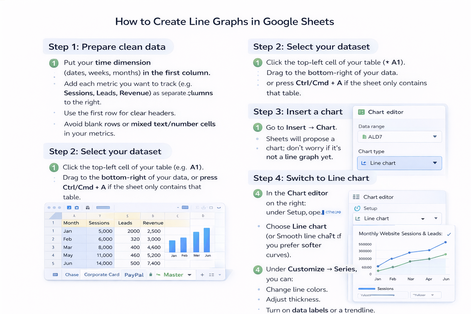
1. Manual Method: Build a Basic Line Graph

Step 1: Prepare clean data

Put your time dimension (dates, weeks, months) in the first column.
Add each metric you want to track (e.g., Sessions, Leads, Revenue) as separate columns to the right.
Use the first row for clear headers.
Avoid blank rows or mixed text/number cells in your metrics.

Step 2: Select your dataset

Click the top‑left cell of your table (e.g., A1).
Drag to the bottom‑right of your data, or press Ctrl/Cmd + A if the sheet only contains that table.

Step 3: Insert a chart

Go to Insert → Chart.
Sheets will propose a chart; don’t worry if it’s not a line graph yet.

Step 4: Switch to Line chart

In the Chart editor on the right, under Setup, open Chart type.
Choose Line chart (or Smooth line chart if you prefer softer curves).
Confirm that your date column is on the horizontal axis and your metrics are on the vertical axis.

Step 5: Customize for clarity

Go to Customize → Chart & axis titles to:
- Rename the chart (e.g., “Monthly Website Sessions & Leads”).
- Add horizontal axis title (e.g., “Month”).
- Add vertical axis title (e.g., “Count of Sessions & Leads”).
Under Customize → Series, you can:
- Change line colors.
- Adjust thickness.
- Turn on data labels or a trendline.

Pros (Manual)

Full control over every visual detail.
Great for learning how charts work.
No extra tools required.

Cons (Manual)

Repetitive: you’ll rebuild or tweak charts every reporting cycle.
Easy to make small mistakes (wrong range, missing months, mislabeled axis).
Scales poorly if you manage many clients, products, or markets.

‍

2. Semi‑Automated: Templates and Sparkline Tricks

If you’re not ready for full AI agents, you can still cut time with built‑in Google Sheets features.

Option A: Reusable chart templates

Create a “master” sheet with your favorite line chart layout.
Use File → Make a copy for each new campaign or client.
Swap in new data under the existing headers; the chart updates automatically.

Option B: SPARKLINE for mini trend lines

In a blank cell, type a formula like:
- =SPARKLINE(B2:G2) where B2:G2 is a row of monthly values.
Sheets renders a tiny line chart in a single cell—perfect for dashboards that compare many products or channels.

Pros (Semi‑Automated)

Faster than rebuilding from scratch.
Keeps visual consistency across reports.
Zero extra tools or setup.

Cons (Semi‑Automated)

You still do the copy‑pasting and data cleanup.
Easy to accidentally break a template by overwriting ranges.
Still not ideal if you handle dozens of Sheets.

‍

3. Fully Automated: Use a Simular AI Computer Agent

Now imagine this weekly scene:

It’s Monday morning. Instead of opening Google Sheets, pasting exports, and fixing chart ranges, you just type: “Update all client performance line graphs for last week and share links in our reporting channel.” Then you watch your AI computer agent do the work.
‍

That’s what Simular Pro is built for: agents that use your desktop and browser like a teammate.

What the agent can do for line graphs

Open your Google Sheets reports in the browser.
Import or paste new data (from CSVs, CRM, ad platforms, etc.).
Clean and format columns so dates, numbers, and headers are consistent.
Insert new line charts or update existing ones when ranges grow.
Apply your standard styling: colors, titles, legends, and axes.
Log every step so you can review and tweak the workflow.

Example: Weekly marketing report automation

Agent downloads the latest ad and analytics exports.
Opens the master reporting Sheet for Client A.
Adds last week’s numbers to the table.
Expands the chart range to include the new rows.
Checks that the correct metrics are on each axis.
Renames the chart subtitle with the latest date range.
Shares the updated Sheet link in your team’s channel.

Pros (AI Agent Automation)

Massive time savings when you have many similar reports.
Production‑grade reliability: Simular agents are designed for workflows with thousands of steps.
Transparent execution: every click and keystroke is inspectable, so you’re never trusting a black box.
Can integrate via webhooks into your existing pipelines (e.g., run after a data refresh completes).

Cons (AI Agent Automation)

Requires a short upfront investment to design and test the workflow.
Best suited when you have recurring tasks (daily/weekly/monthly), not one‑off charts.
You still own the logic: you decide which Sheets, metrics, and timelines matter.

‍

4. When Should You Hand It Off to an Agent?

If you answer “yes” to any of these, it’s time to delegate:

You recreate the same Google Sheets line graphs every week.
You manage multiple clients or product lines with similar dashboards.
Reporting prep steals time from strategy, sales, or creative work.

In that world, your best move isn’t to click faster—it’s to let a Simular AI computer agent click for you, exactly the way you would, while you focus on what the chart is trying to tell you.

Scale Google Sheets Line Graphs With AI Agents Now

Train Simular agent

Define a clear playbook for your Simular AI agent: which Google Sheets to open, which ranges hold date and metric columns, and how each line graph should be styled and titled.

Test and refine agent

Run your Simular AI agent on a copy of your Google Sheets reports first. Verify data ranges, axes, and labels, then tweak its instructions until the line graphs update flawlessly.

Scale tasks to agent

Once the workflow is solid, delegate all recurring Google Sheets reporting to your Simular AI agent. It can update line graphs across clients and teams on a schedule or via webhook triggers.